Note

Download full notebook here

2-D CARMApy

CARMApy also has a 2-D mode, as described in Powell and Zhang (2024). It works by advecting the entire cloud column at a constant longitudinal wind speed along the equator while allowing the temperature structure to vary by longitude. To tell CARMApy that the model is a 2-D one, set the flag is_2d=True when calling the carmapy.Carma() constructor.

import carmapy
from matplotlib import pyplot as plt
import numpy as np

carma = carmapy.Carma("2d_carmapy", is_2d=True)

# carma.set_stepping(dt=5000, output_gap=1000, n_tstep=250000)
carma.set_stepping(dt=5000, output_gap=249999, n_tstep=250000)

Note that for this model it runs for far longer than a 1-D model as it takes longer to converge (note that this model is for demonstation purposes only—it should not be necessarily considered to be converged).

CARMApy also provides sample atmospheric profiles for an example 2-D CARMApy run. These profiles are taken from GCM simulations of sub-neptunes in Steinrueck et al. (2024)

P_levs, T_levs, kzz_levs, longitudes = carmapy.example.example_2d_levels()

carma.add_P(P_levs)
carma.add_T(T_levs)
carma.add_kzz(kzz_levs)

Note that unlike in the 1-D model, T_levs is a 2-D array of shape (NZ, NLONGITUDE)

We can now set the physical parameters of the atmosphere. The surface gravity, mean molecular weight, and metallicity are set as before. We also now must set the average logitudinal wind velocity velocity_avg and the radius of the planet r_planet. By default all of these quantities are in cgs units but we can use the use_jovian_radius=True flag to instead specify the planetary radius in Jovian radii

carma.set_physical_params(
    surface_grav = 1060,
    wt_mol=28.7,
    log_metallicity=3.5,
    velocity_avg=1e5,
    r_planet=0.25,
    use_jovian_radius=True
)
carma.set_atmospheric_parameters_from_defaults("Pure H2")

Having specified the physical parameters and the non-z atmospheric profile, we can now tell CARMApy to calculate the z coordinate profile of the atmosphere.

WARNING: Unlike in a 1-D run, the z-coordinate does not correspond to a cartesian altitude, it instead is a log pressure coordinate which is equal to the longitudinally averaged scale height at the base of the atmosphere multiplied by the absolute value of the log ratio of the pressure coordinate to the pressure at the base of the atmosphere. It is reccomended to just use carma.calculate_z() for this calculation

carma.calculate_z()

We will now add the cloud groups to our model. As this is a cooler model than our example 1-D model, we will be adding KCl as a homogeneously nucleating species and ZnS as a species that can heterogeneously nucleate on KCl. Note that populate_abundances_at_cloud_base() determines the cloud base from a longitudinally averaged P-T profile

carma.add_hom_group("KCl", 1e-8)
carma.add_het_group("ZnS", "KCl", 1e-8 * 2**(1/3))
carmapy.chemistry.populate_abundances_at_cloud_base(carma)

We can now run our model. This run should take 20-60 min depending on your computer (The carma.run() command is commented out as it takes too long to run when compiling the documentation—if you are following along you should uncomment that piece of code)

# carma.run()

For 2-D CARMApy in particular it is reccomended to restart a longer run but with dense output frequency to ensure that you can get output data for the entire planet at a similar time. Setting the carma.restart=1 flag tells the model to continue from the last saved model state instead of starting from a blank slate atmosphere again

carma.restart=1
carma.set_stepping(dt=800, output_gap=1, n_tstep=3000)
# carma.run(suppress_output=True)

As before, we can read our results with carmapy.read_results()

carma.read_results(read_diag=True)

Plotting our results is very similar to in 1-D CARMApy. Because it is often desired to plot results as a function of longitude instead of timestep, for 2-D runs CARMApy provides the function carma.results.longitude_map(). This function takes in a 3-D array of shape (NZ, NBIN, NT) and transforms it to an array of shape (NZ, NBIN, NLONGITUDE) where each longitude bin in the average of all timesteps corresponding to that longitude. This function is designed to work on the "numden" array as well as any of the microphysical rates arrays

import matplotlib
import matplotlib.pyplot as plt
import numpy as np

species = "Pure KCl"

t_step = -1

density = np.nansum(carma.results.longitude_map(carma.results.clouds[species]["numden"]), axis=1)

max_den = np.nanmax(density)

levels = np.logspace(int(np.log10(max_den) + 1)-10, int(np.log10(max_den) + 1), 21)

plt.contourf(longitudes,
             carma.results.P,
             density + 1e-100,
             norm=matplotlib.colors.LogNorm(vmin=levels.min(), vmax=levels.max()),
             levels=levels,
             extend="min")

plt.plot(np.ones(carma.results.P.shape) * -90, carma.results.P, 'r--')
plt.plot(np.ones(carma.results.P.shape) * 90, carma.results.P, 'r--')

plt.yscale("log")
plt.gca().invert_yaxis()

plt.ylabel("Pressure [baryes]")
plt.xlabel("Longitude [degrees]")


plt.colorbar(label="Number Density (cm⁻³)")
plt.title(species)
plt.show()

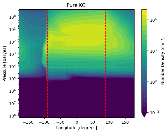
As you can see, most of the cloud formation occurs on the dayside of the planet (between the two dashed-red lines). Note that the periodic beating with longitude is unlikely to be physical—it can be reduced by increasing the number of timesteps averaged over.

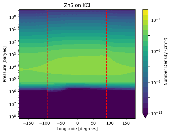
As before, we can also make this plot for Zns on KCl clouds

species = "ZnS on KCl"

t_step = -1

density = np.nansum(carma.results.longitude_map(carma.results.clouds[species]["numden"]), axis=1)

max_den = np.nanmax(density)

levels = np.logspace(int(np.log10(max_den) + 1)-10, int(np.log10(max_den) + 1), 21)

plt.contourf(longitudes,
             carma.results.P,
             density + 1e-100,
             norm=matplotlib.colors.LogNorm(vmin=levels.min(), vmax=levels.max()),
             levels=levels,
             extend="min")

plt.plot(np.ones(carma.results.P.shape) * -90, carma.results.P, 'r--')
plt.plot(np.ones(carma.results.P.shape) * 90, carma.results.P, 'r--')

plt.yscale("log")
plt.gca().invert_yaxis()

plt.ylabel("Pressure [baryes]")
plt.xlabel("Longitude [degrees]")


plt.colorbar(label="Number Density (cm⁻³)")
plt.title(species)
plt.show()

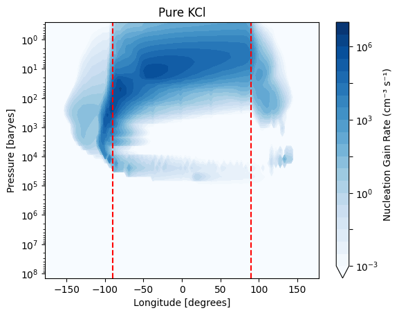
As mentioned before, the longitude_map() function also works for microphysical rates

species = "Pure KCl"

t_step = -1

density = np.nansum(carma.results.longitude_map(carma.results.clouds[species]["grow_gain_rate"]), axis=1)

max_den = np.nanmax(density)

levels = np.logspace(int(np.log10(max_den) + 1)-10, int(np.log10(max_den) + 1), 21)

plt.contourf(longitudes,
             carma.results.P,
             density + 1e-100,
             norm=matplotlib.colors.LogNorm(vmin=levels.min(), vmax=levels.max()),
             levels=levels,
             extend="min",
             cmap="Blues")

plt.plot(np.ones(carma.results.P.shape) * -90, carma.results.P, 'r--')
plt.plot(np.ones(carma.results.P.shape) * 90, carma.results.P, 'r--')

plt.yscale("log")
plt.gca().invert_yaxis()

plt.ylabel("Pressure [baryes]")
plt.xlabel("Longitude [degrees]")


plt.colorbar(label="Nucleation Gain Rate (cm⁻³ s⁻¹)")
plt.title(species)
plt.show()