Note

Download full notebook here

Reading CARMA Results

To begin reading results, we can start by loading the carmapy object that we created in the previous tutorial.

import carmapy

carma = carmapy.load_carma("my_first_carma")

Note that carmapy.load_carma() only loads in the initial conditions of the carma run, not the results. To also load the results we can run the following code:

carma.read_results(read_diag=True)

Using the read_diag=True flag allows us to read in the microphysical rates and core mass fraction (see below) at the expense of taking significantly longer to read in results. The difference here is not that high but for larger results files it can be reasonably substantial

Ensuring Convergence

When drawing conclusions from carma results, it is critical to first ensure that the model has converged. The fastest way to check convergence in carma is the check to see how the gas abundance at the top of the atmosphere has been changing—if the gas abundance for each species has reached a steady or stable oscillatory state, carma is most likely converged. carmapy includes a convinience function that plots the gas abundance at the top of the atmosphere for you:

carma.results.plot_toa_gas(burn_in=0)

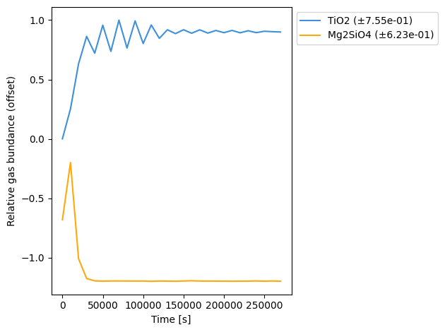
As the graphs are saturated by the peak at the beginning of the simulation, we can adjust the burn_in parameter to exclude the first few samples from our plot

carma.results.plot_toa_gas(burn_in=8)

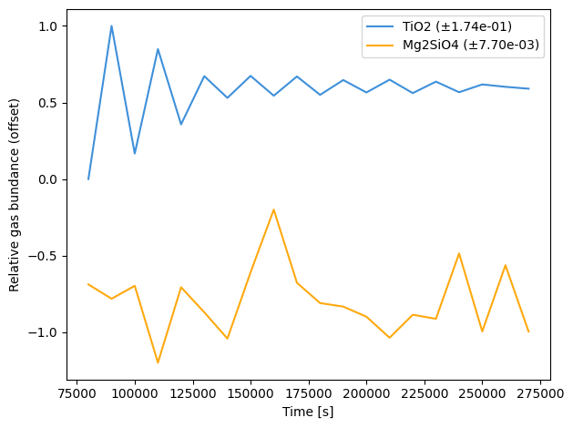
This model is plausibly converged but it would likely be useful to run it for longer to ensure convergence

Accessing and Plotting Cloud Model Results

Cloud model results are provided in a dictionary carma.results.clouds. Note as a single gas species can both homogeneously and heterogeneously condence, and could theoretically heterogeneously condense onto multiple different seed particles, carmapy automatically adjusts the names of each cloud species to distinguish between these cases:

1. If a cloud species is homogeneously nucleated from a gas species, then the name of the cloud species is “Pure <gas species name>” (ie “Pure TiO2”)

2. If a cloud species is formed from a the heterogeneous nucleation of a gas species onto an existing cloud particle then the cloud species name is “<gas species name> on <seed particle gas name>” (ie “Mg2SiO4 on TiO2”)

To see the names of all of the cloud species in a given carma run you can run:

carma.results.clouds.keys()

dict_keys(['Pure TiO2', 'Mg2SiO4 on TiO2'])

For each cloud species we store a number items, 3 of which are listed below:

1. numden: a \(n_z \times n_r \times n_t\) numpy array that represents the number density of particles in units of cm⁻³ where \(n_z\) is the number of atmospheric “centers” (see the previous tutorial for the distinction between “centers” and “levels”) and the first element in that axis corresponds to the bottom of the atmosphere, \(n_r\) is the number of size bins with the first element in that axis corresponding to the minimum particle size for the species, and \(n_t\) being the number of output steps, with the first element in that axis corresponding to the first output of the simulation

2. r: a numpy array with \(n_r\) elements which correspond to the radius, in cm, of each particle size bin

3. r_mass a numpy array with \(n_r\) elements which correspond to the mass of particles in each radius bin

Using this output, you can plot the number density profile of TiO2 as follows:

import matplotlib
import matplotlib.pyplot as plt
import numpy as np

t_step = -1

max_den = np.max(carma.results.clouds["Pure TiO2"]["numden"][:,:,t_step])

levels = np.logspace(int(np.log10(max_den) + 1)-10, int(np.log10(max_den) + 1), 21)

plt.contourf(carma.results.clouds["Pure TiO2"]["r"],
             carma.results.P,
             carma.results.clouds["Pure TiO2"]["numden"][:, :, t_step] + 1e-100,
             norm=matplotlib.colors.LogNorm(vmin=levels.min(), vmax=levels.max()),
             levels=levels,
             extend="min")

plt.xscale("log")
plt.yscale("log")
plt.gca().invert_yaxis()

plt.ylabel("Pressure [baryes]")
plt.xlabel("Particle Radius [cm]")


plt.colorbar(label="Number Density (cm⁻³)")
plt.title("TiO2")
plt.show()

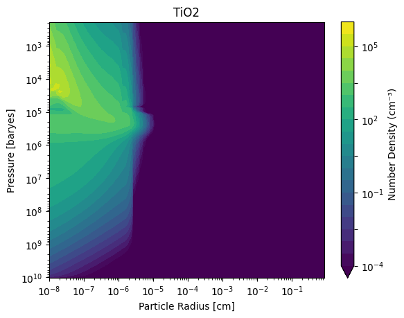
Notice that here we use carma.results.P which gives the pressures the results are calculated at. Under normal use of carmapy, this should be equivalent to carma.results.P_centers once results are loaded.

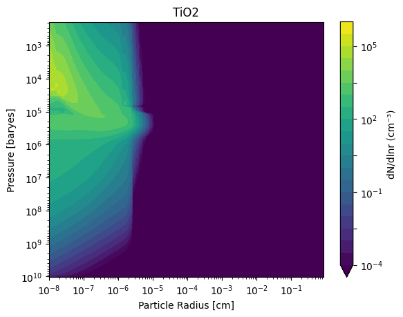
Note that CARMA outputs number densities not :math:`dN/dln r`. If you instead wanted to plot that you can divide the number densityies by the ratio between subsequent bins, which is a constant for CARMA runs. For example:

t_step = -1
r = carma.results.clouds["Pure TiO2"]["r"]

dlnr =r[1] / r[0]

max_den = np.max(carma.results.clouds["Pure TiO2"]["numden"][:,:,t_step]/dlnr)

levels = np.logspace(int(np.log10(max_den) + 1)-10, int(np.log10(max_den) + 1), 21)

plt.contourf(carma.results.clouds["Pure TiO2"]["r"],
             carma.results.P,
             (carma.results.clouds["Pure TiO2"]["numden"][:, :, t_step]/dlnr + 1e-100),
             norm=matplotlib.colors.LogNorm(vmin=levels.min(), vmax=levels.max()),
             levels=levels,
             extend="min")

plt.xscale("log")
plt.yscale("log")
plt.gca().invert_yaxis()

plt.ylabel("Pressure [baryes]")
plt.xlabel("Particle Radius [cm]")


plt.colorbar(label="dN/dlnr (cm⁻³)")
plt.title("TiO2")
plt.show()

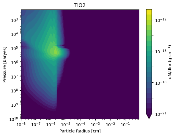
If instead of number density, you wanted to plot the mass density of the clouds you can do so by multiplying the number density array by the r_mass array. For example:

t_step = -1
r = carma.results.clouds["Pure TiO2"]["r"]

dlnr = r[1] / r[0]

mass_density = (carma.results.clouds["Pure TiO2"]["numden"][:,:,t_step]
                * carma.results.clouds["Pure TiO2"]["r_mass"]
                / dlnr
                + 1e-100)

max_den = np.max(mass_density)

levels = np.logspace(int(np.log10(max_den) + 1)-10, int(np.log10(max_den) + 1), 21)

plt.contourf(carma.results.clouds["Pure TiO2"]["r"],
             carma.results.P,
             mass_density,
             norm=matplotlib.colors.LogNorm(vmin=levels.min(), vmax=levels.max()),
             levels=levels,
             extend="min")

plt.xscale("log")
plt.yscale("log")
plt.gca().invert_yaxis()

plt.ylabel("Pressure [baryes]")
plt.xlabel("Particle Radius [cm]")


plt.colorbar(label="dM/dlnr (g cm⁻³)")
plt.title("TiO2")

plt.show()

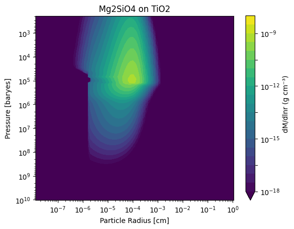
For completeness, here is the same plot but instead for the Mg₂SiO₄ on TiO₂ clouds:

t_step = -1
r = carma.results.clouds["Mg2SiO4 on TiO2"]["r"]

dlnr = r[1] / r[0]

mass_density = (carma.results.clouds["Mg2SiO4 on TiO2"]["numden"][:,:,t_step]
                * carma.results.clouds["Mg2SiO4 on TiO2"]["r_mass"]
                / dlnr
                + 1e-100)

max_den = np.max(mass_density)

levels = np.logspace(int(np.log10(max_den) + 1)-10, int(np.log10(max_den) + 1), 21)

plt.contourf(carma.results.clouds["Mg2SiO4 on TiO2"]["r"],
             carma.results.P,
             mass_density,
             norm=matplotlib.colors.LogNorm(vmin=levels.min(), vmax=levels.max()),
             levels=levels,
             extend="min")

plt.xscale("log")
plt.yscale("log")
plt.gca().invert_yaxis()

plt.ylabel("Pressure [baryes]")
plt.xlabel("Particle Radius [cm]")


plt.colorbar(label="dM/dlnr (g cm⁻³)")
plt.title("Mg2SiO4 on TiO2")

plt.show()

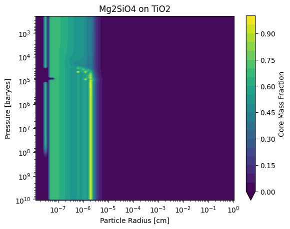
Accessing Core Mass Fraction

If we want to determine what fraction of heterogeneous cloud particles consists of the core “seed” particle, we can access that with another field of the carma.results.clouds dictionary, specifically with the "coremass_frac" key. Visually, we can access and plot it as follows:

t_step = -1
r = carma.results.clouds["Mg2SiO4 on TiO2"]["r"]

dlnr = r[1] / r[0]

mass_density = (carma.results.clouds["Mg2SiO4 on TiO2"]["coremass_frac"][:,:,t_step]
                + 1e-100)

max_den = np.max(mass_density)

levels = np.linspace(0, 1, 21)

plt.contourf(carma.results.clouds["Mg2SiO4 on TiO2"]["r"],
             carma.results.P,
             mass_density,
             norm=matplotlib.colors.Normalize(vmin=levels.min(), vmax=levels.max()),
             levels=levels,
             extend="min")

plt.xscale("log")
plt.yscale("log")
plt.gca().invert_yaxis()

plt.ylabel("Pressure [baryes]")
plt.xlabel("Particle Radius [cm]")


plt.colorbar(label="Core Mass Fraction")
plt.title("Mg2SiO4 on TiO2")

plt.show()

Accessing and Ploting Gas Resevoir Abundances

The gas abundances for each species are stored in an dictionary carma.results.gasses where you can index the dictionary by gas names. For example. carma.results.gasses["TiO2"] is a \(n_z \times n_t\) array which stores the number mixing ratio of TiO₂ at each z-center and time-step in units of parts-per-million (ppm). You can access and plot the gas profiles as follows:

NT = -1

plt.plot(carma.results.gases["TiO2"][:, NT-1], carma.results.P, label="TiO2 (g)")
plt.plot(carma.results.gases["Mg2SiO4"][:, NT-1], carma.results.P, label="Mg (g)")

plt.xscale("log")
plt.yscale("log")
plt.gca().invert_yaxis()

plt.legend()
plt.ylabel("Pressure [barye]")
plt.xlabel("Gas Abundance [ppm]")

plt.show()

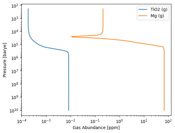
Note that the gas abundance is constant below the cloud base and then is depleted where the cloud formation occurs.

Plotting Microphysical Rates

The carma.results.clouds dictionary also stores a number of microphysical rates (all in units of particles/s/cm³):

• nuc_gain_rate stores the gross (not net) gain in particles in a bin due to both heterogeneous and homogeneous nucleation

• nuc_loss_rate stores the gross (not net) loss in particles in a bin due to both heterogeneous nucleation (homogeneous nucleation does not deplete the particles in any bin)

• grow_gain_rate stores the gross (not net) gain in particles in a bin due to condensational growth

• grow_loss_rate stores the gross (not net) loss of particles in a bin due to condensational growth (ie if a particle from bin a grows such that it is now in bin b, that would be considered a loss due to growth for bin a)

• evap_gain_rate stores the gross (not net) gain in particles in a bin due to evaporation (ie if a particle from bin b evaporates such that it is now in bin a, that would be considered a gain due to evaporation for bin a)

• evap_loss_rate stores the gross (not net) loss in particles in a bin due to evaporation

Note that due to conservation of mass, at a particular timestep and for a given condensate grow_gain_rate - grow_loss_rate = evap_gain_rate - evap_loss_rate = 0 (but not nuc_gain_rate+nuc_loss_rate)

The code below shows how to access and plot these quantities for Pure TiO₂

t_step = -1
species = "Pure TiO2"

fig, axs = plt.subplots(2, 3, sharex=True, sharey=True, figsize=(12,5))

r = carma.results.clouds[species]["r"]

dlnr = r[1] / r[0]

quantities = ["nuc_gain_rate", "nuc_loss_rate", "grow_gain_rate",
              "grow_loss_rate", "evap_gain_rate", "evap_loss_rate"]

cmaps = ["Blues", "Purples", "Reds"]

for i in range(6):
    ax_x = i % 2
    ax_y = int(i / 2)
    ax = axs[ax_x, ax_y]

    values = (carma.results.clouds[species][quantities[i]][:,:,t_step] + 1e-100)

    max_val= np.max(values)

    levels = np.logspace(int(np.log10(max_val) + 1)-10, int(np.log10(max_val) + 1), 21)

    cmap = ax.contourf(carma.results.clouds[species]["r"],
                carma.results.P,
                values,
                norm=matplotlib.colors.LogNorm(vmin=levels.min(), vmax=levels.max()),
                levels=levels,
                cmap = cmaps[ax_y],
                extend="min")

    plt.xscale("log")
    plt.yscale("log")
    plt.ylim(1e8, 1e3)

    if ax_y == 0: ax.set_ylabel("Pressure [baryes]")
    if ax_x == 1: ax.set_xlabel("Particle Radius [cm]")

    ax.set_title(quantities[i])
    plt.colorbar(cmap)

plt.show()

/var/folders/b5/mg6kqfls38ng45s7mny2b0nr0000gp/T/ipykernel_24102/1456181699.py:26: UserWarning: Log scale: values of z <= 0 have been masked
  cmap = ax.contourf(carma.results.clouds[species]["r"],

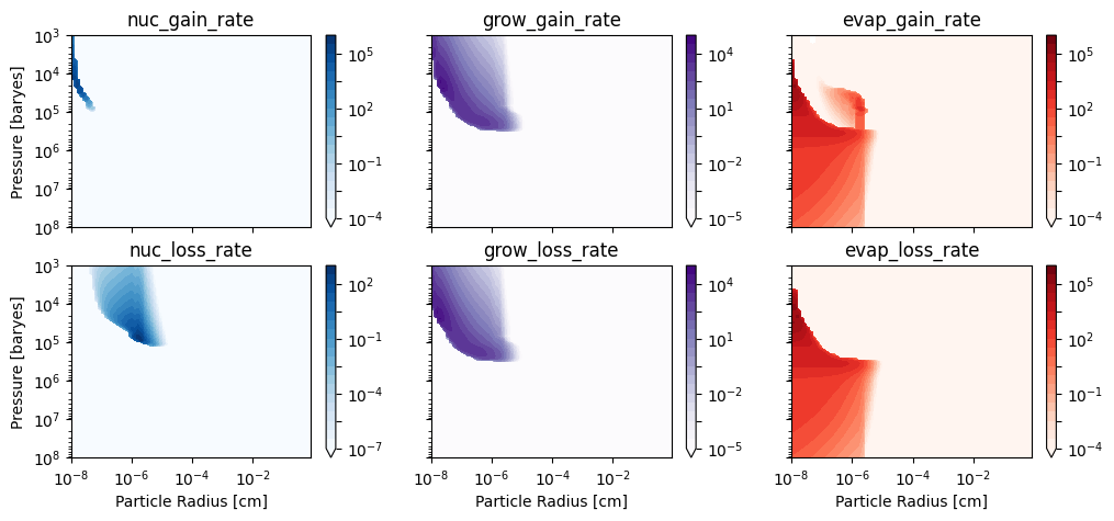
Note that the growth (and evaporation) loss and gain rate plots look incredibly similar—this is because particles most often move into nearby bins when growing or evaporation so the location of gain and loss will be similar in both locations on this plot.

We can create similar plots for Mg₂SiO₄ on TiO₂:

t_step = -1
species = "Mg2SiO4 on TiO2"

fig, axs = plt.subplots(2, 3, sharex=True, sharey=True, figsize=(12,5))

r = carma.results.clouds[species]["r"]

dlnr = r[1] / r[0]

quantities = ["nuc_gain_rate", "nuc_loss_rate", "grow_gain_rate",
              "grow_loss_rate", "evap_gain_rate", "evap_loss_rate"]

cmaps = ["Blues", "Purples", "Reds"]

for i in range(6):
    ax_x = i % 2
    ax_y = int(i / 2)
    ax = axs[ax_x, ax_y]

    values = (carma.results.clouds[species][quantities[i]][:,:,t_step] + 1e-100)

    max_val= np.max(values)

    levels = np.logspace(int(np.log10(max_val) + 1)-10, int(np.log10(max_val) + 1), 21)

    cmap = ax.contourf(carma.results.clouds[species]["r"],
                carma.results.P,
                values,
                norm=matplotlib.colors.LogNorm(vmin=levels.min(), vmax=levels.max()),
                levels=levels,
                cmap = cmaps[ax_y],
                extend="min")

    plt.xscale("log")
    plt.yscale("log")
    plt.ylim(1e8, 1e3)


    if ax_y == 0: ax.set_ylabel("Pressure [baryes]")
    if ax_x == 1: ax.set_xlabel("Particle Radius [cm]")

    ax.set_title(quantities[i])
    plt.colorbar(cmap)

plt.show()

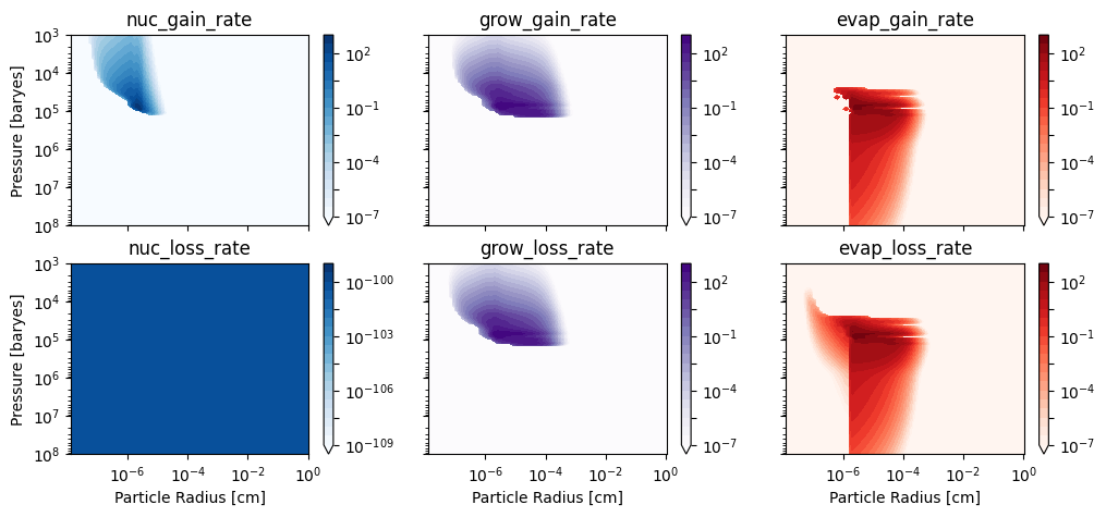
Note that there is no nucleation loss rate as there is no particles nucleating on the Mg₂SiO₄ on TiO₂ Cloud particles