Note

Download full notebook here

2-D CARMApy

Running 2D CARMApy

CARMApy also has a 2-D mode, as described in Powell and Zhang (2024). It works by advecting the entire cloud column at a constant longitudinal wind speed along the equator while allowing the temperature structure to vary by longitude. To tell CARMApy that the model is a 2-D one, set the flag is_2d=True when calling the carmapy.Carma() constructor.

import carmapy
from matplotlib import pyplot as plt
import numpy as np
import warnings
import os


carma = carmapy.Carma("2d_carmapy", is_2d=True)
carma.set_stepping(dt=2500, output_gap=249999, n_tstep=1_000_000)

Note that for this model it runs for far longer than a 1-D model as it takes longer to converge (note that this model is for demonstration purposes only—it should not necessarily be considered to be converged).

CARMApy also provides sample atmospheric profiles for an example 2-D CARMApy run. The bundled profile is a hot Jupiter (Teq = 1800 K, log g = 3.3 cgs, Rp = 1.3 Rjup, solar metallicity) derived from a GCM grid and latitude-averaged over |lat| ≤ 20°. example_2d_levels() returns the pressure (barye), temperature (NZ × NLON, K), Kzz (cm²/s, from Moses et al. 2021 Eq 1 with a 10¹¹ cm²/s ceiling), zonal wind speed (NZ × NLON, cm/s), and longitudes (degrees).

P_levs, T_levs, kzz_levs, U_levs, longitudes = carmapy.example.example_2d_levels()

carma.add_P(P_levs)
carma.add_T(T_levs)
carma.add_kzz(kzz_levs)

Note that unlike in the 1-D model, T_levs is a 2-D array of shape (NZ, NLONGITUDE).

We can now set the physical parameters of the atmosphere. The surface gravity, mean molecular weight, and metallicity are set as before. We also now must set the average longitudinal wind velocity velocity_avg and the radius of the planet r_planet. By default all of these quantities are in cgs units but we can use the use_jovian_radius=True flag to instead specify the planetary radius in Jovian radii. For velocity_avg we use the mean |U| at 1 mbar from the GCM-derived wind profile.

z_wind = int(np.argmin(np.abs(P_levs - 1e3)))  # 1 mbar = 1e3 barye
velocity_avg = float(np.mean(np.abs(U_levs[z_wind, :])))

carma.set_physical_params(
    surface_grav=10**(1.3 + 2),   # log g = 1.3 (SI) → cgs
    wt_mol=2.3,
    log_metallicity=0.0,
    velocity_avg=velocity_avg,
    r_planet=1.3,
    use_jovian_radius=True,
)
carma.set_atmospheric_parameters_from_defaults("Pure H2")

Having specified the physical parameters and the non-z atmospheric profile, we can now tell CARMApy to calculate the z coordinate profile of the atmosphere.

WARNING: Unlike in a 1-D run, the z-coordinate does not correspond to a Cartesian altitude — it is instead a log pressure coordinate equal to the longitudinally averaged scale height at the base of the atmosphere multiplied by the absolute value of the log ratio of the pressure coordinate to the pressure at the base of the atmosphere. It is recommended to just use carma.calculate_z() for this calculation.

carma.calculate_z()
carma.extend_atmosphere(1e11)

We will now add the cloud groups to our model. For this hot Jupiter we add TiO2 as a homogeneously nucleating species and Mg2SiO4 as a species that can heterogeneously nucleate on TiO2. Note that populate_abundances_at_cloud_base() determines the cloud base from a longitudinally averaged P-T profile.

carma.add_hom_group("TiO2", 1e-8)
carma.add_het_group("Mg2SiO4", "TiO2", 1e-8 * 2**(1/3))
carmapy.chemistry.populate_abundances_at_cloud_base(carma)

We can now run our model. This run should take 20-60 min depending on your computer.

carma.run(suppress_output=True)

For 2-D CARMApy in particular it is recommended to restart a longer run with dense output frequency to ensure that you can get output data for the entire planet at a similar time. Setting the carma.restart=1 flag tells the model to continue from the last saved model state instead of starting from a blank atmosphere again.

carma.restart=1
carma.set_stepping(dt=800, output_gap=1, n_tstep=1500)
carma.run()

As before, we can read our results with carma.read_results()

carma.read_results(read_diag=True)

2D CARMApy Results

Plotting our results is very similar to in 1-D CARMApy. Because it is often desired to plot results as a function of longitude instead of timestep, for 2-D runs CARMApy provides the function carma.results.longitude_map(). This function takes a 3-D array of shape (NZ, NBIN, NT) and transforms it to an array of shape (NZ, NBIN, NLONGITUDE) where each longitude bin is the average of all timesteps corresponding to that longitude. This function is designed to work on the "numden" array as well as any of the microphysical rates arrays.

import matplotlib
import matplotlib.pyplot as plt
import numpy as np

species = "Pure TiO2"

t_step = -1

density = np.nansum(carma.results.longitude_map(carma.results.clouds[species]["numden"]), axis=1)

max_den = np.nanmax(density)

levels = np.logspace(int(np.log10(max_den) + 1)-10, int(np.log10(max_den) + 1), 21)

plt.contourf(longitudes,
             carma.results.P,
             density + 1e-100,
             norm=matplotlib.colors.LogNorm(vmin=levels.min(), vmax=levels.max()),
             levels=levels,
             extend="min")

plt.plot(np.ones(carma.results.P.shape) * -90, carma.results.P, 'r--')
plt.plot(np.ones(carma.results.P.shape) * 90, carma.results.P, 'r--')

plt.yscale("log")
plt.gca().invert_yaxis()

plt.ylabel("Pressure [baryes]")
plt.xlabel("Longitude [degrees]")


plt.colorbar(label="Number Density (cm⁻³)")
plt.title(species)
plt.show()

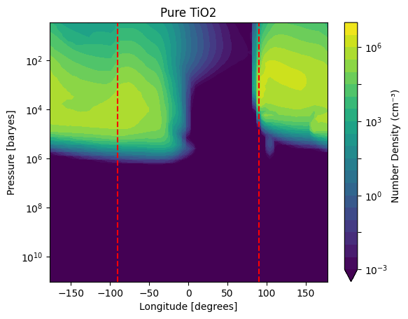
As you can see, most of the cloud formation occurs on the dayside of the planet (between the two dashed-red lines). Note that the periodic beating with longitude is unlikely to be physical—it can be reduced by increasing the number of timesteps averaged over.

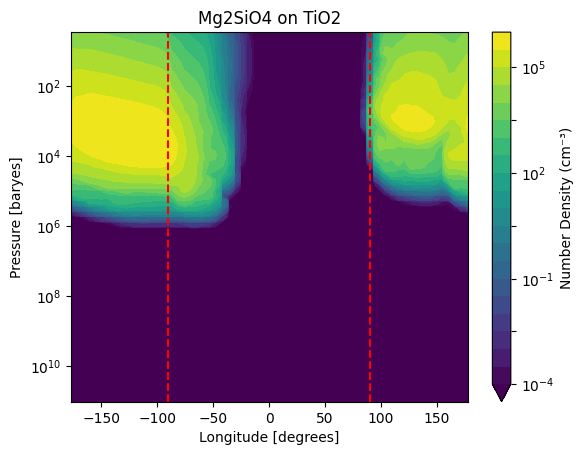
As before, we can also make this plot for Mg2SiO4 on TiO2 clouds:

species = "Mg2SiO4 on TiO2"

t_step = -1

density = np.nansum(carma.results.longitude_map(carma.results.clouds[species]["numden"]), axis=1)

max_den = np.nanmax(density)

levels = np.logspace(int(np.log10(max_den) + 1)-10, int(np.log10(max_den) + 1), 21)

plt.contourf(longitudes,
             carma.results.P,
             density + 1e-100,
             norm=matplotlib.colors.LogNorm(vmin=levels.min(), vmax=levels.max()),
             levels=levels,
             extend="min")

plt.plot(np.ones(carma.results.P.shape) * -90, carma.results.P, 'r--')
plt.plot(np.ones(carma.results.P.shape) * 90, carma.results.P, 'r--')

plt.yscale("log")
plt.gca().invert_yaxis()

plt.ylabel("Pressure [baryes]")
plt.xlabel("Longitude [degrees]")


plt.colorbar(label="Number Density (cm⁻³)")
plt.title(species)
plt.show()

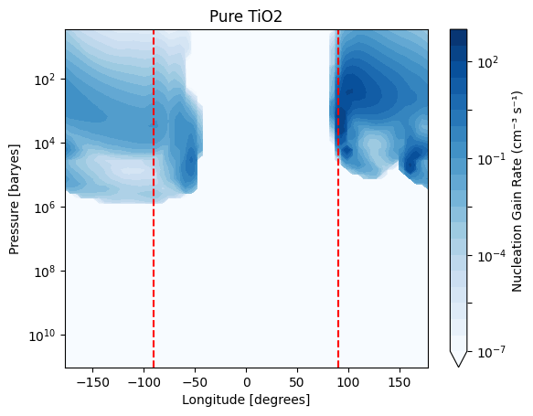
As mentioned before, the longitude_map() function also works for microphysical rates:

species = "Pure TiO2"

t_step = -1

density = np.nansum(carma.results.longitude_map(carma.results.clouds[species]["grow_gain_rate"]), axis=1)

max_den = np.nanmax(density)

levels = np.logspace(int(np.log10(max_den) + 1)-10, int(np.log10(max_den) + 1), 21)

plt.contourf(longitudes,
             carma.results.P,
             density + 1e-100,
             norm=matplotlib.colors.LogNorm(vmin=levels.min(), vmax=levels.max()),
             levels=levels,
             extend="min",
             cmap="Blues")

plt.plot(np.ones(carma.results.P.shape) * -90, carma.results.P, 'r--')
plt.plot(np.ones(carma.results.P.shape) * 90, carma.results.P, 'r--')

plt.yscale("log")
plt.gca().invert_yaxis()

plt.ylabel("Pressure [baryes]")
plt.xlabel("Longitude [degrees]")


plt.colorbar(label="Nucleation Gain Rate (cm⁻³ s⁻¹)")
plt.title(species)
plt.show()

Limb-Asymmetric Transmission Spectra

2D CARMApy gives us the ability to look at longitudinal variations in observables. One example of this is CARMApy is able to create spectra that show the difference between the morning terminator and the evening terminator

As covered in tutorial 3, gen_picaso_atm_file() and gen_picaso_cloud_file() write the atmosphere and cloud input files that PICASO needs. For 2-D runs both methods require a longitude index, which selects the temperature profile and the time-averaged cloud number density for that longitude column.

Note: this section requires PICASO to be installed and configured (see https://natashabatalha.github.io/picaso/installation.html). The PYSYN_CDBS and picaso_refdata environment variables must be set before importing PICASO, either in your shell rc or inline in the cell below.

# This section expects `picaso_refdata` and `PYSYN_CDBS` to already be set in
# your environment (e.g. in your shell rc). If you'd rather set them inline,
# uncomment and edit:
# path = '/path/to/picaso/reference'
# os.environ['picaso_refdata'] = path
# os.environ['PYSYN_CDBS'] = path

from picaso import justdoit as jdi

# Identify the longitude indices closest to the morning and evening limbs
morning_idx = int(np.argmin(np.abs(longitudes + 90)))
evening_idx = int(np.argmin(np.abs(longitudes -   90)))

print(f"Morning limb: lon = {longitudes[morning_idx]:.1f}°  (index {morning_idx})")
print(f"Evening limb: lon = {longitudes[evening_idx]:.1f}°  (index {evening_idx})")

out_dir = os.path.join(carma.name, "picaso_outputs")
os.makedirs(out_dir, exist_ok=True)

λs = np.linspace(1e-4, 2e-3, 1000)  # cm — wavelength grid for Mie scattering

for label, idx in [("morning", morning_idx), ("evening", evening_idx)]:
    carma.results.gen_picaso_atm_file(
        file_path=os.path.join(out_dir, f"fastchem_{label}.atm"),
        longitude=idx,
    )
    carma.results.gen_picaso_cloud_file(
        λs,
        file_path=os.path.join(out_dir, f"clouds_{label}.atm"),
        longitude=idx,
    )

WARNING: Failed to load Vega spectrum from None; Functionality involving Vega will be severely limited: FileNotFoundError(2, 'No such file or directory') [stsynphot.spectrum]

Morning limb: lon = -92.8°  (index 15)
Evening limb: lon = 87.2°  (index 47)
Wrote file: 2d_carmapy/picaso_outputs/fastchem_morning.atm
Wrote file: 2d_carmapy/picaso_outputs/clouds_morning.atm
Wrote file: 2d_carmapy/picaso_outputs/fastchem_evening.atm
Wrote file: 2d_carmapy/picaso_outputs/clouds_evening.atm

With the PICASO input files written, we can compute the transmission spectra. The main difference between this and tutorial 3 is that these are transmission spectra so we need to specify the star properties.

Teq   = 1800.0  # K (from example_2d_levels profile)
log_met = 0.0

GRAV_CONST = 6.674e-8  # cm^3 g^-1 s^-2
Mp  = carma.surface_grav * carma.r_planet**2 / GRAV_CONST

opa   = jdi.opannection(wave_range=[0.5, 15])
R_BIN = 500


def compute_transmission(atm_path, cloud_path):
    case = jdi.inputs(calculation="transmission")
    case.phase_angle(0)
    case.gravity(
        mass=Mp, mass_unit=jdi.u.Unit("g"),
        radius=carma.r_planet, radius_unit=jdi.u.Unit("cm"),
    )

    case.star(opa, 6500, 0.0, 4.2, radius=1.5, radius_unit=jdi.u.Unit("R_sun"),
              database="phoenix")

    case.atmosphere(filename=atm_path, sep=r"\s+")
    case.clouds(filename=cloud_path, sep=r"\s+")

    df = case.spectrum(opa, full_output=True, calculation="transmission")

    wno, rprs2 = df["wavenumber"], df["transit_depth"]
    wno_bin, rprs2_bin = jdi.mean_regrid(wno, rprs2, R=R_BIN)

    return 1e4 / wno_bin, rprs2_bin * 1e6   # µm, ppm


print("Computing morning limb spectrum...")
λ_morning, depth_morning = compute_transmission(
    os.path.join(out_dir, "fastchem_morning.atm"),
    os.path.join(out_dir, "clouds_morning.atm"),
)

print("Computing evening limb spectrum...")
λ_evening, depth_evening = compute_transmission(
    os.path.join(out_dir, "fastchem_evening.atm"),
    os.path.join(out_dir, "clouds_evening.atm"),
)

depth_combined = 0.5 * (depth_morning + depth_evening)

Computing morning limb spectrum...
Computing evening limb spectrum...

We can now plot our spectra:

fig, ax = plt.subplots(figsize=(12, 4.5))

ax.plot(λ_morning,  depth_morning,  color="#3f90da", lw=2,
        label="Morning limb", alpha=0.85)
ax.plot(λ_evening,  depth_evening,  color="#bd1f01", lw=2,
        label="Evening limb", alpha=0.85)
ax.plot(λ_morning,  depth_combined, color="gray",    lw=1,
        label="Combined")

ax.set_xlabel("Wavelength [µm]")
ax.set_ylabel("Transit Depth [ppm]")
ax.set_xlim(0.5, 15)
ax.legend(framealpha=0.9)


fig.tight_layout()
plt.show()

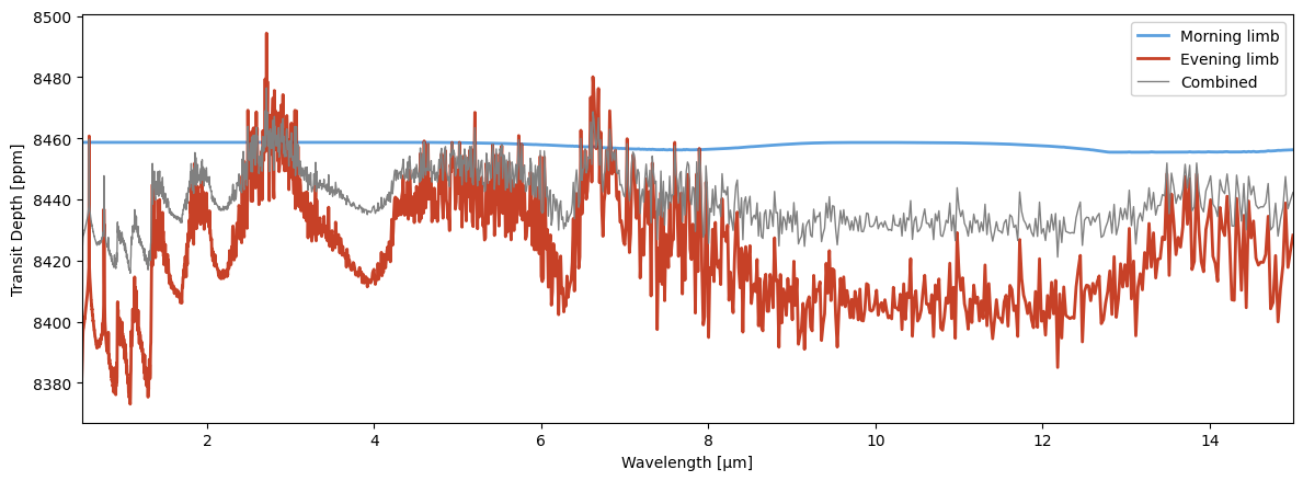
As you can see, the morning spectrum is a lot flatter than the evening spectrum. If you look up to where we plotted number densities earlier, you can see that the morning limb is a lot cloudier than the evening limb – this is what creates the flatter morning spectrum

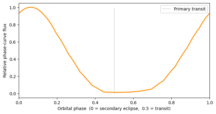
Thermal Emission Phase Curve

Another observable that 2-D CARMApy enables is the thermal emission phase curve, which tracks how the thermal flux from the planet changes as it orbits its star and different longitudes rotate into view.

Note: because this requires one PICASO run per sampled longitude, this section can take several minutes to run.

band_range    = (2.0, 4.0)    # µm
n_phase       = 200           # number of orbital phase points
stride        = 4

lon_idxs = np.arange(0, carma.NLONGITUDE, stride)
lons = longitudes[lon_idxs]
dlon        = 360.0 / len(lon_idxs)

lambdas = np.linspace(1e-4, 1e-3, 1000)  # cloud file wavelength grid
opa_thermal = jdi.opannection(wave_range=list(band_range))

We loop over the sampled longitude columns, write the PICASO input files, run the thermal spectrum, and integrate the flux over the 2–4 µm band.

band_flux = np.zeros(len(lon_idxs))

for k, ilong in enumerate(lon_idxs):
    atm_path = os.path.join(out_dir, f"fastchem_lon{ilong:2d}.atm")
    cloud_path = os.path.join(out_dir, f"clouds_lon{ilong:2d}.atm")

    carma.results.gen_picaso_atm_file(file_path=atm_path, longitude=ilong,
                                      suppress_output=True)
    carma.results.gen_picaso_cloud_file(lambdas, file_path=cloud_path, longitude=ilong,
                                        suppress_output=True)

    case = jdi.inputs(calculation="thermal")

    case.phase_angle(0)
    case.gravity(gravity=carma.surface_grav, gravity_unit=jdi.u.Unit("cm/(s**2)"),
                 radius=carma.r_planet, radius_unit=jdi.u.Unit("cm"))

    case.star(opa_thermal, 6500, 0.0, 4.2,
              radius=1.5, radius_unit=jdi.u.Unit("R_sun"), database="phoenix")

    case.atmosphere(filename=atm_path, sep=r"\s+")
    case.clouds(filename=cloud_path, sep=r"\s+")

    with warnings.catch_warnings(): # supress picaso warnings
        warnings.simplefilter("ignore")

        df = case.spectrum(opa_thermal, full_output=True, calculation="thermal")
        wno = np.asarray(df["wavenumber"])
        fp  = np.asarray(df["thermal"])

        order   = np.argsort(wno)
        wno, fp = wno[order], fp[order]

        ls  = 1e4 / wno
        mask    = (ls >= band_range[0]) & (ls <= band_range[1])
        band_flux[k] = np.trapezoid(fp[mask], wno[mask])

Now that we have spectra at each of the sampled longitude points, we can create a phase curve. Each visible point on the planet will contribute a flux proportional to the cosine of the angle of the line of sight to the normal

phase       = np.linspace(0.0, 1.0, n_phase)
lon_obs = 360.0 * phase


mu         = np.cos((lons[None, :] - lon_obs[:, None])*np.pi/180)   # (N_PHASE, N_LON)
weight     = np.clip(mu, 0.0, None) * 2 * np.pi / len(lons)

phase_flux = np.sum(band_flux[None, :] * weight, axis=1)
phase_norm = phase_flux / phase_flux.max()

contrast = phase_flux.max() / max(phase_flux.min(), 1e-30)

plt.subplots(figsize=(8, 4))

plt.plot(phase, phase_norm, color="darkorange", lw=2)

plt.plot([0.5, 0.5], [0, 1], ls=":", color="grey", lw=1, label="Primary transit")

plt.xlabel("Orbital phase  (0 = secondary eclipse,  0.5 = transit)")
plt.ylabel("Relative phase-curve flux")

plt.xlim(0, 1)
plt.legend(framealpha=0.9)

fig.tight_layout()
plt.show()