Note

Download full notebook here

Creating Spectra with Picaso

carmapy has a few built-in functions that make it easier to collate the results of a carma simulation into a form usable by picaso. Picaso (natashabatalha/picaso) is a python package that, among other things, has tools for creating exoplanet and brown dwarf emission spectra. This tutorial assumes that you have already installed picaso and configured your environment variables to point to the references folder (see https://natashabatalha.github.io/picaso/installation.html). Alternatively you can uncomment the lines below which set the environment variables and adjust the path if you don’t have them already configured. To check that picaso is installed and configured properly run the following code:

import os
import picaso

# This notebook expects `picaso_refdata` and `PYSYN_CDBS` to already be set in
# your environment (e.g. in your shell rc). If you'd rather set them inline,
# uncomment and edit:
# path = '/path/to/picaso/reference'
# os.environ['picaso_refdata'] = path
# os.environ['PYSYN_CDBS'] = path

Now let’s import picaso submodules and carmapy, and load our data again

import numpy as np
from matplotlib import pyplot as plt

from picaso import justdoit as jdi
from picaso import justplotit as jpi

import carmapy

jpi.output_notebook()

carma = carmapy.load_carma("my_first_carma")
carma.read_results()

WARNING: Failed to load Vega spectrum from None; Functionality involving Vega will be severely limited: FileNotFoundError(2, 'No such file or directory') [stsynphot.spectrum]

Loading BokehJS ...

Next, let us set up picaso to generate the spectra of free-floating brown dwarfs in thermal emission. If you wish to instead look at a planet orbiting a star, look at the picaso tutorials for that case and modify the below code appropriately.

opacity = jdi.opannection(wave_range=[.5,15])
example_case = jdi.inputs(calculation='browndwarf')
example_case.phase_angle(0)

We now tell carma to calculate the atmospheric and cloud optical properties and pass those numbers to picaso:

λs = np.linspace(5e-4, 2e-3, 1000)

carma.results.gen_picaso_atm_file()
carma.results.gen_picaso_cloud_file(λs)

example_case.gravity(gravity=carma.surface_grav,
                     gravity_unit=jdi.u.Unit('cm/(s**2)'))

example_case.atmosphere(filename=f'{carma.name}/fastchem.atm', sep='\\s+')
example_case.clouds(filename=f"{carma.name}/clouds.atm", sep='\\s+')

Wrote file: my_first_carma/fastchem.atm
Wrote file: my_first_carma/clouds.atm

We can now calculate and then bin the spectrum as follows

df = example_case.spectrum(opacity, full_output=True,calculation='thermal') #note the new last key

R = 1000
wno, fp = df['wavenumber'] , df['thermal']
wno_bin, fp_bin = jdi.mean_regrid(wno, fp, R=R)

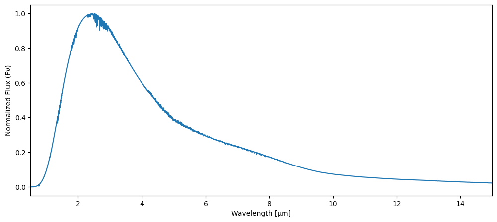
And here is an example of how to plot the spectrum

fig, ax = plt.subplots(figsize=(12, 5))

λ = 1e4/wno_bin
plt.plot(λ, fp_bin/np.max(fp_bin))

plt.xlabel("Wavelength [μm]")
plt.ylabel("Normalized Flux (Fν)")
plt.xlim(.5, 15)
plt.show()

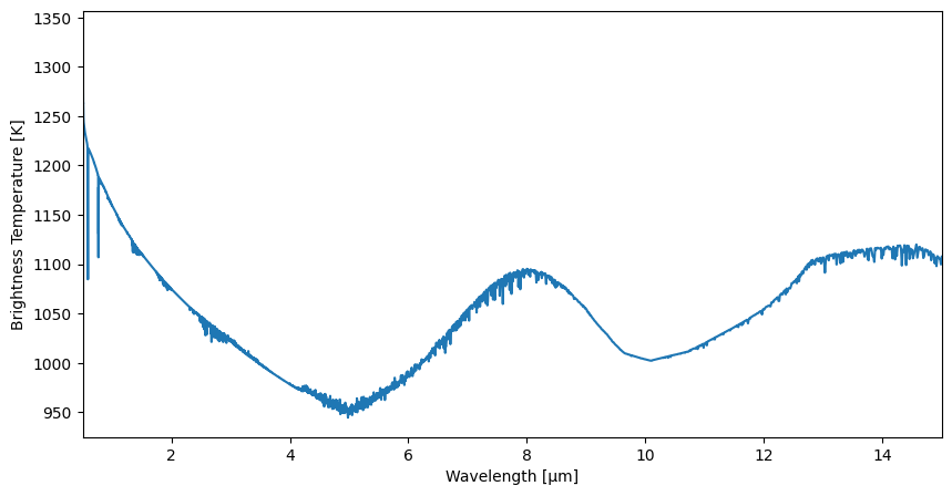
Similarly, here is the spectrum instead plotted as brightness temperature

fig, ax = plt.subplots(figsize=(10, 5))


λ = 1e4/wno_bin
T = jpi.brightness_temperature({"wavenumber": wno,
                                "thermal": fp},
                                R=R,
                                plot=False)

plt.plot(λ, T)

plt.xlabel("Wavelength [μm]")
plt.ylabel("Brightness Temperature [K]")
plt.xlim(.5, 15)
plt.show()